Product Development: The Optimizer’s Curse

Over the past eight years, the ROI of late-stage development investments, estimated for 12 large-cap pharmaceutical companies, declined from 10% to 2%.¹ Certainly, companies are not advancing compounds that they forecast to return a measly 2%. When evaluated after Phase II clinical trials, the advancing compounds looked like champions, with some of them even booked as blockbusters; so why did they arrive downstream as duds?

The common explanation is biased evaluations, overconfidence in the likelihood of FDA approval, and overestimates of potential profits. If you expunge these biases, downstream disappointment will disappear. This reasoning is wrong.

Even if the evaluations are unbiased,  there will still be disappointment suffered downstream. The problem is selection, sequencing, and resource allocation—all the things called portfolio management. Portfolio management creates optimism, fooling analysts because of a subtle but ubiquitous phenomenon, the optimizer’s curse, which raises expectations while insidiously reducing results.

Pharmaceutical executives do not know of the optimizer’s curse, even though this phenomenon creates overvalued drug development portfolios while reducing portfolio value. In academia, the optimizer’s curse is becoming an important part of the project portfolio management literature. While the problem is well-known in financial portfolio management and by executives who manage portfolios of oil and gas exploration assets,² shouldn’t pharma executives learn of this destructive problem and the remedies available to defeat it?

How cunningly deceitful is the curse? Based on industry data, focusing on the selection of compounds to advance to Phase III, a rough but reasonable estimate suggests that forecasts of blockbuster profits are, on average, 100% too high. Meanwhile, estimates of Phase III’s expected net present value (eNPV) are, on average, 25% to 45% too high. (The eNPV is the probability of technical success multiplied by the net present value, NPV, of the profits a compound produces if it is launched.)

How can unbiased data overvalue Phase III drugs?

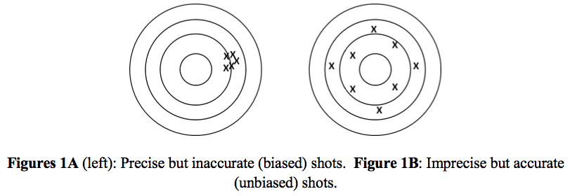
Let’s begin with the definitions of inaccuracy and imprecision. Figure 1A below presents arrows on a target, tightly clustered, but off to the right. Tight clustering indicates precision, aiming with a steady hand that produces only small random errors. The rightward shift, because the bow’s sights are off, affects all arrows. It is inaccuracy, or synonymously, bias. Figure 1B presents imprecision, a dispersed pattern, caused by an unsteady hand that imparts large random errors into every shot. Because the cluster is centered on the bullseye, the shots are accurate, or equivalently, unbiased.

Evaluations made immediately after compounds complete Phase II are always imprecise. Forecasting the NPV of future profits, contingent on a compound’s FDA approval, requires extrapolating years into the future, anchoring predictions to uncertain estimates of safety and efficacy, while grappling with dynamic competitive and regulatory landscapes.

In their famous paper, “The optimizer’s curse: Skepticism and post-decision surprise in decision analysis,” scholars Smith and Winkler show how imprecise project evaluations affect project selection. Suppose you can choose one of two projects, and to make the example compelling, assume they have the same NPV. You evaluate the projects accurately (unbiased) but imprecisely. Each assessment has a 50% chance of being optimistic and a 50% chance of being pessimistic. Four possible outcomes exist:

• You underestimate the value of both projects (25% chance).
• You overestimate the value of one project and underestimate the value of the other one (50% chance).
• You overestimate the value of both projects (25% chance).
• You select the project with the highest estimated value, so 75% of the time you overestimate the worth of your investment. 

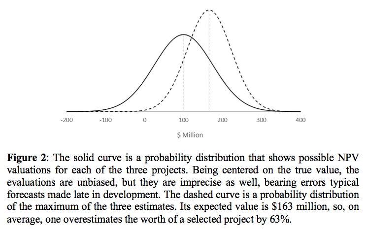
Now suppose you select one of three projects, and to make a vivid case, they are worth the same amount: $100 million. Your evaluations are accurate (unbiased), but imprecision is 75%, equaling the erroneous forecasts found towards the end of drug development.³ Figure 2 below reveals the results. The solid curve is a probability distribution of the possible evaluations of each project, centered on $100 million (unbiased) but with a standard deviation (imprecision) of $75 million. The dashed curve is a probability distribution showing the possible values of the highest estimate. Its mean is $163 million. Even though your valuations are unbiased, you choose the project with the highest estimate, which overstates its value, on average, by 63% ($63 million).

Imprecision overvalues some compounds while undervaluing others. Portfolio management exploits these errors to create overvalued portfolios while destroying value, sometimes by advancing overvalued jokers, other times by canceling undervalued aces. These problems plague all selection methods, including rankings, portfolio optimization, and simulation optimization. However, some methods suffer the optimizer’s curse worse than others.

How bad is the optimizer’s curse?

A compound completes Phase II, successfully, so you estimate the NPV of the profits it will produce if it achieves FDA approval. Producing cheers from your colleagues, you announce a forecast for blockbuster profits. Now you ask yourself, “Considering the imprecision in my forecast, how does a prediction of blockbuster profits arise?” It occurs in one of two ways: (1) the compound is indeed a blockbuster and the forecasting error is small or (2) the compound is not a blockbuster and the forecasting error is large and optimistic. Most drugs have below-average profits, while only a few are blockbusters, so the second possibility is more likely.

In analogy, suppose your scientists develop a diagnostic test for a rare disease, a disease that afflicts one of every one hundred people. The test has a negligible false-negative rate and a false-positive rate of 5%. In a hundred tests, you expect to get one true-positive and five-false-positives, so a person diagnosed with the disease has only a 17% chance (1/6) of having the disease. Because the disease is rare, a positive test is likely to be a false-positive.  Similarly, so many compounds make meager profits, while so few become blockbusters, that a forecast of blockbuster sales is likely to be a false-positive. On average, forecasts of blockbuster returns are optimistic.

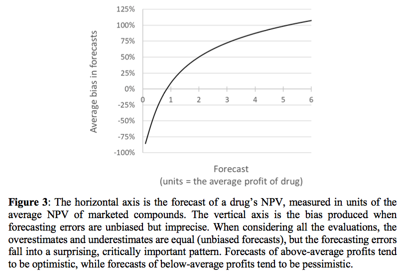
We can estimate this optimism with industry data. We start with a highly skewed distribution, one that accurately represents the distribution of pharmaceutical profits. We randomly sample thousands of values from this distribution, with each sample representing one drug. To each sample, we add a forecasting error, randomly selecting the error from a distribution that is symmetrical and centered on zero, thus ensuring unbiased errors.  Further, we give this distribution a standard deviation to match the forecasting errors found downstream in development. Finally, we scale the error, so small markets have smaller forecasting errors than larger markets. For example, overestimating price by 10% creates a larger forecasting error in a $100 million market than in a $10 million market. We now have thousands of “drugs” with true profits and forecasts, and we ask, “For drugs forecasted to be blockbusters, what is the average true profit?  Figure 3 presents the surprising results, with these two highlights:

• Even though the forecasting errors are unbiased, the errors occur in a striking pattern. Compounds predicted to produce above-average returns are, on average, overestimates. Forecasts predicted to produce below-average returns are, on average, underestimates.
• If we define blockbusters as compounds having five times the average profit for a drug, forecasts of blockbuster profits, on average, are 100% too high.

Now ask yourself, “Which compounds advance to Phase III?” Most of the advancing compounds have high forecasts. Simulation studies suggest that, after adjusting for Phase III failures rates and development costs, the compounds advancing to Phase III are overvalued by 25% to 45%.

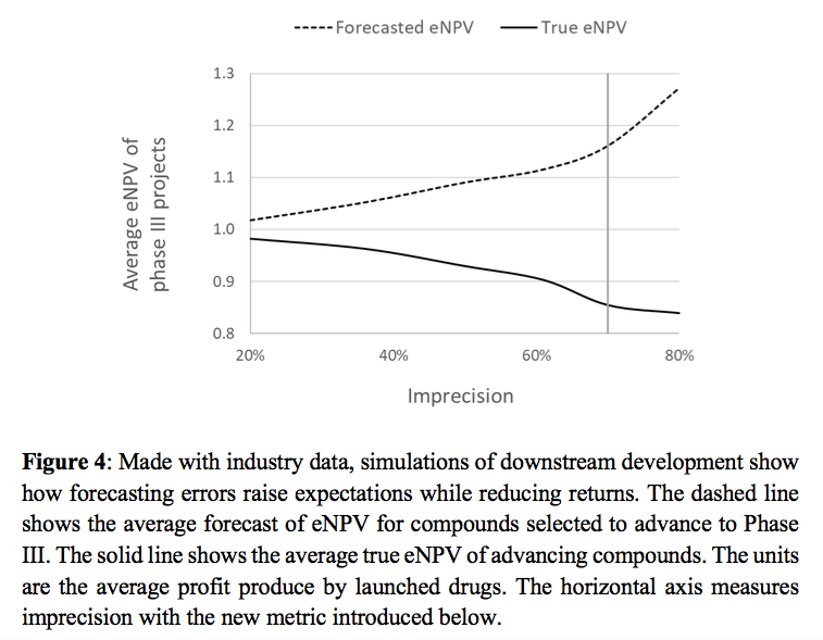
Figure 4 shows the impact of imprecision by comparing expectations of Phase III’s value to the phase’s true value.  As forecasts of NPV becomes less precise, project selection errors become more numerous, more frequently sending overvalued compounds downstream and more consistently canceling lucrative but undervalued drugs.  Expectations rise only to be dashed by downstream results.

How to mitigate the optimizer’s curse

How can you mitigate the optimizer’s curse?  Nobel Laureate Daniel Kahneman presented a general approach for improving forecasts, which using some theory of the optimizer’s curse, we can adapt to propose a simple, and hopefully robust, method.⁴ Every compound is a member of a class, defined by therapeutic area, new molecular entity, or me-too drug, and other distinctions. Estimate the average net present value for the drugs in a compound’s class, NPV_CA.  Then combine the class average with a compound’s forecasted net present value, NPV_F, to create a new forecast: NPV_New = εNPV_CA + (1 - ε)NPV_F. The calculation, a weighted average, adjusts a compound’s forecast toward its class average. Applied to multiple forecasts, it reduces high estimates while levitating low estimates, thus flattening the curve in Figure 3, which shrinks imprecision. Conceptually, averaging imbibes an estimate with additional information, comingling two distinct points of view, which resolves uncertainty and makes forecasts more precise.

The weight, ε, a new metric, measures imprecision. You estimate ε by focusing on the drugs in a compound’s class. From industrywide databases, retrieve the forecasts of NPV made when these drugs were still in development, such as forecasts made by sell-side analysts. Calculate the variance of these forecasts, Var(Forecasts).  Then for each of these compounds, calculate the NPV of the profits the compounds realized after launch. You may need to forecast the sales remaining in the compounds’ product lifecycles.  Finally, calculate the variance of these realized profits, Var(Realized). The ratio 1 - ε = Var(Realized)/Var(Forecasts), which should always be between 0% and 100%, is the percentage of the forecasts that is signal. Its compliment, ε, is the percentage of the forecasts that is noise. (A few adjustments, too technical to mention here, will improve your estimate of ε.  Additionally, if 1 - ε >100%, your forecasting methods are too coarse, engaging too few factors or too little information.

With an alternative approach, based on academic models, but still using industry data, I calculated 67% <  ε < 76% for compounds that have just finished Phase II. Only 20% to 33% of forecasts made immediately after Phase II was signal, an outstandingly low number. This prodigious imprecision is why the fall from expectations to results, from Phase II to Phase III, is so severe, and why, as Figure 4 suggests, imprecise forecasts depress Phase III value by more than 10%.

To test the above technique, which you should do before using it, calculate ε as described above. Then adjust the historical forecasts with the weighted average technique. Specifically, letting NPV_H denote the historical forecasts, calculate NPV_New = εNPV_CA + (1 - ε)NPV_H. Now calculate Var(Forecasts) for NPV_New, and, finally, recalculate ε using 1 - ε = Var(Realized)/Var(Forecasts). By how much did ε decrease? If the reduction in imprecision is substantial and 1 - ε  < 100%, the adjustment worked. Use it to improve your forecasts.

Managing extended uncertainty

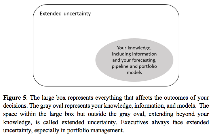
The optimizer’s curse is an example of a pervasive problem: extended uncertainty. As Figure 5 illustrates, your knowledge, being partial and imperfect, covers only a fraction of the factors that affect results. The unknown and imperfectly known issues are called extended uncertainty because they extend beyond your knowledge.

Managing extended uncertainty is critical to success, and two general approaches can help you.  First, uncertainty affects results, so its fingerprints mark outcomes, highlighting mistaken assumptions, identifying misleading information, and revealing unknown-unknowns. Analyzing results, actions best described as analytics for portfolio management, will help you diminish extended uncertainty and advance mediocre decision methods into industry leading champions.

Second, when extended uncertainty is extreme, decision strategies that explicitly maximize value falter.  In these situations, practices that reduce the cost of negatives outcomes will perform better. In Figure 4, the vertical line, estimated via simulation, demarks the transition.  For ε < 70% (to the left of the line) portfolio optimization, maximizing eNPV is the best decision method. For ε  > 70%, forecasts of eNPV are so erroneous that other methods outperform portfolio optimization. These approaches build good choice sets, exploit whatever data is reliable, exclude noisy data, simplify models and decision methods, and where possible, increase flexibility. The threshold of ε  > 70% depends largely on the average profit and average cost from developing one new drug. You can estimate a range of ε in which the transition occurs for your pipeline. Then estimate ε for each phase of development.  Phases with values of ε below the transition, likely Phase III, and possibly Phase II as well, benefit by decision methods that maximize value.  Phases further upstream, including discovery, will benefit from the alternative approaches.

Beyond the noise

In drug development, some executives might dismiss downstream disappointment as a mere misfortune, but if Phase III consistently underperforms, the failure arises not from chance but the optimizer’s curse. Selection advances the compounds with the highest evaluations, but, on average, some of this value is ethereal. It is comprised of unfounded optimism, the unwanted residue of imperfect assumptions and noisy data, two blemishes that afflict all forecasts. When reality removes the false optimism, results disappoint.

Fortunately, you can mitigate the optimizer’s curse by integrating forecasts with their class averages.  Additionally, analyzing results, carefully finding the fingerprints of extended uncertainty, will identify the malign issues that harm your decision methods. You can then adjust your practices to create robust, successful portfolio management.

Gary Summers is President and Founder, Pipeline Physics, LLC

References

1. Steedman, M., K. Taylor, M. Stockbridge, C. Korba, S. Shah, M. Thaxter, “Unlocking R&D productivity: Measuring the return from pharmaceutical innovation 2018.” Deloitte Centre for Health Solutions, Deloitte LLP Life Sciences and Health Care Practices.

2. Presentations of the optimizer’s curse in the oil and gas industry include Chen, M. and J. Dyer, “Inevitable disappointment in projects selected on the basis of forecasts,” SPE Journal, 2009, vol. 14, no. 2, pp. 216-221.  Schuyler, J. and T. Nieman, “Optimizer’s curse: removing the effect of this bias in portfolio planning,” SPE Projects Facilities Construction, 2008 vol. 3, no. 1, pp. 1-9.  Begg, S. and R. Bratvold (2008), “Systematic prediction errors in oil and gas project and portfolio selection.

3. Cha, Rifia, and Sarraf, “Pharmaceutical forecasting: throwing darts?” Nature Reviews Drug Discovery, 2013, vol. 12, no. 10, pp. 737-738.

4. Lovallo and Kahneman, “Delusions of success – how optimism undermines executives’ decisions,” Harvard Business Review, 2003, vol. 81, no. 7, pp. 56-63.

Source